计算物理第七次作业
Problem 4.9
In this section we saw that orbits are unstable for any value of
that is not precisely 2 in (4.12). A related question, which we did not address (until now), is how unstable an orbit might be. That is, how long will it take for an unstable orbit to become obvious. The answer to this question depends on the nature of the orbit. If the initial velocity is chosen so as to make the orbit precisely circular, then the value of in (4.12) will make absolutely no difference. Of course, in practice it is impossible to construct an orbit that is exactly circular, so the instabilities when will always be apparent given enough time. Even so, orbits that start out as nearly circular will remain almost stable for a longer period than those that are highly elliptical. Investigate this by studying orbits with the same value of (say, ) and comparing the hebavior with different values of the ellipticity of the orbit. You should find that the orientation of orbits that are more nearly circular will rotate more slowly than those that are highly elliptical. (尝试利用不是2的 值构造圆形轨道,并讨论各种不同轨道情况下的稳定性。)
根据伟大的牛顿万有引力公式
我们可以直接写出有心力场下行星的运动方程:
太阳系中,我们令距离单位为天文单位,时间单位为年,可以得到
下面我们简单模拟一下不同偏心率轨道的运动,验证模拟的精度是足够的,可以近似为一条重叠的轨道。
%matplotlib inline
import matplotlib.pyplot as pl
import numpy as np
from math import *

class solar_system(object):
    def __init__(self, eccentricity = 0, initial_x = 1., beta = 2, total_time = 20, time_step = 0.001, alpha = 0):
        self.beta = beta
        self.e = eccentricity
        self.t = np.arange(time_step, total_time + time_step, time_step)
        self.dt = time_step
        self.alpha = alpha
        self.x = initial_x

    def run(self):
        # 这里我们固定起始位置,并且根据偏心率直接给出可以形成闭合轨道的初始速度
        self.x = np.array([self.x])
        self.y = np.array([0])
        self.v_x = np.array([0])
        self.v_y = np.array([2 * pi * sqrt((1 - self.e)/(1 + self.e))])
        self.r = np.array([])
        for t in self.t:
            self.r = np.append(self.r, sqrt(self.x[-1]**2 + self.y[-1]**2))
            self.v_x = np.append(self.v_x, (self.v_x[-1] - self.dt * (4*pi**2 * self.x[-1] / self.r[-1] ** (self.beta + 1) * (1 + self.alpha / self.r[-1] ** 2))))
            self.v_y = np.append(self.v_y, (self.v_y[-1] - self.dt * (4*pi**2 * self.y[-1] / self.r[-1] ** (self.beta + 1) * (1 + self.alpha / self.r[-1] ** 2))))
            self.x = np.append(self.x, (self.x[-1] + self.v_x[-1] * self.dt))
            self.y = np.append(self.y, (self.y[-1] + self.v_y[-1] * self.dt))


    def show(self, k):
        pl.subplot(k)
        pl.subplots_adjust(wspace = 0.3)
        pl.plot(self.x, self.y, linewidth = 1)
        pl.plot(0, 0, 'ro', markersize = 10)
        pl.xlabel('x (AU)')
        pl.ylabel('y (AU)')
        pl.xlim(-1.2, 1.2)
        pl.ylim(-1.2, 1.2)
        pl.title(r'Planetary Orbits  $\beta = %.2f\qquad e = %.2f$'% (self.beta, self.e))

if __name__ == '__main__':
    pl.figure(figsize = (12,4), dpi=80)
    k = 131
    for e in (0, 0.2, 0.3):
        a = solar_system(eccentricity = e)
        a.run()
        a.show(k)
        k += 1
    pl.show()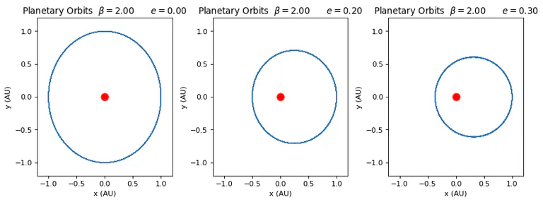
可以看到在此时的精度下轨迹可以近似认为是重合的轨迹(当然放大后仍然会发现有抖动),下面我们研究一下在
for i in (2.01, 2.05, 2.1, 2.3):
    k = 141
    pl.figure(figsize = (16.9, 4), dpi=80)
    for e in(0, 0.1, 0.2, 0.5):
        a = solar_system(beta = i, eccentricity = e)
        a.run()
        a.show(k)
        k += 1
    pl.show()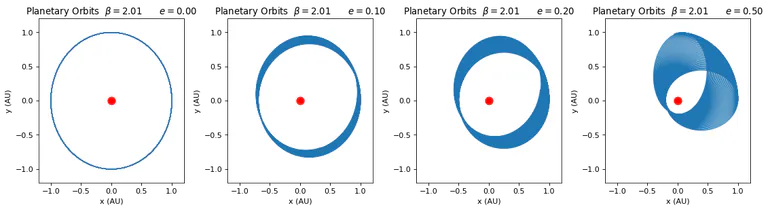
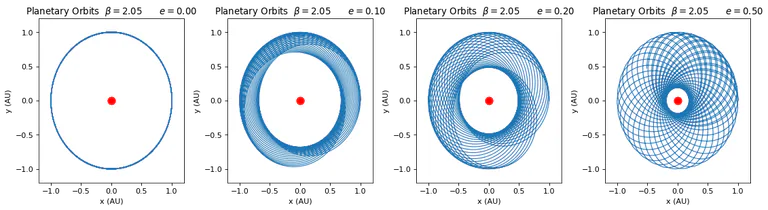
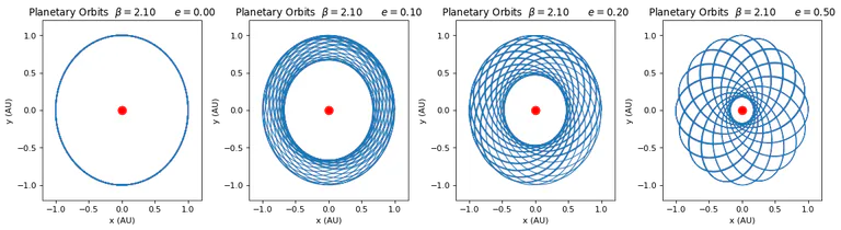
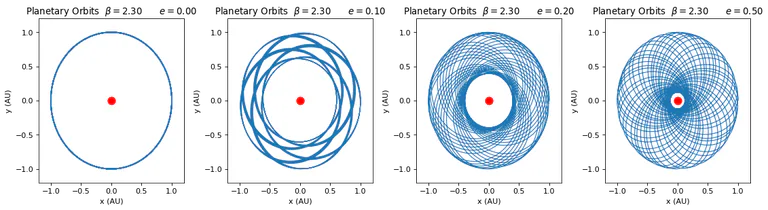
可以发现和题目叙述相同,对于圆形轨道,即使
但是当轨道的偏心率不为0时,即使对于
而且可以发现,当偏心率越大,轨道的进动速度越快,这应该是很容易理解的,偏心率越大意味着轨道越椭圆,其近日点和远日点的差距也就越大,从而使得轨道的进动更加迅速。
Problem 4.11
Investigate how the precession of the perihelion of a planet’s orbit due to general relativity varies as a function of the eccentricity of the orbit. Study the precession of different elliptical orbits with different eccentricities, but with the same value of the perihelion. Let the perihelion have the same value as for Mercury, so that you can compare it with the results shown in this section. (比较相同近地点情况下进动的速率。)
广义相对论下,对万有引力公式有近似的修正
利用广义相对论的修正,可以很好地解释水星的轨道进动现象,下面我们进行一下简单的模拟。这里由于
class Mercury(solar_system):
    def precession(self):
        diff = np.diff(np.sign(np.diff(self.r))) # 寻找近地点
        locations = np.where(diff == 2)[0] + 1
        self.need_r = self.r[locations]
        self.need_x = self.x[locations]
        self.need_y = self.y[locations]
        self.need_t = self.t[locations]
        self.theta = np.arccos(self.need_x / self.need_r) * 180 / pi
        # self.theta[self.need_y < 0] = 360 - self.theta[self.need_y < 0]
        # self.theta = np.abs(self.theta - 180)
        self.func = np.polyfit(self.need_t, self.theta, 1) # 最小二乘法线性拟合
        self.y_fit = self.func[0] * self.need_t + self.func[1]

    def show(self):
        pl.plot(self.need_t, self.theta, 'o', markersize = 4)
        pl.plot(self.need_t, self.y_fit, linewidth = 1.5, label = r'$e=%.2f\quad\omega=%.3f$'% (self.e, self.func[0]))
        pl.xlabel('t (yr)')
        pl.ylabel(r'$\theta(^\circ)$')
        pl.title(r'Oribit orientation versus time $\alpha = %.4f$'% self.alpha)

if __name__ == '__main__':
    pl.figure(figsize = (8, 8), dpi=80)
    for i in (0.1, 0.15, 0.2, 0.25):
        a = Mercury(alpha=0.0008, eccentricity = i, initial_x = (1+i)/(1-i), total_time = 5, time_step = 0.0001)
        a.run()
        a.precession()
        a.show()
    pl.legend(loc = 'lower right')
    pl.show()
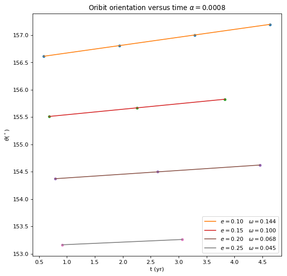
可以发现,轨道进动的速度随着偏心率的增大而减小,但可以看出并不是线性关系,下面取更多数据进行一下计算。(时间不够没模拟出来