计算物理第八次作业
4.19
Study the behavior of our model for Hyperion for different initial conditions. Estimate the Lyapunov exponent from calculation of
, such as those shown in Figure 4.19. Examine how this exponent varies as a function of the eccentricity of the orbit.
import numpy as np
import matplotlib.pyplot as pl
from math import *

class hyperion(object):
    def __init__(self, eccentricity = 0, initial_theta = 0, total_time = 10, time_step = 0.0001):
        self.e = eccentricity
        self.t = np.arange(time_step, total_time + time_step, time_step)
        self.dt = time_step
        self.theta = initial_theta

    def run(self):
        self.x = np.array([1])
        self.y = np.array([0])
        self.v_x = np.array([0])
        self.v_y = np.array([2 * pi * sqrt((1 - self.e)/(1 + self.e))])
        self.w = np.array([0])
        self.theta = np.array([self.theta])
        self.theta_raw = np.array([self.theta])
        self.r = np.array([sqrt(self.x ** 2 + self.y ** 2)])
        for n in range(len(self.t) - 1):
            temp_r = sqrt(self.x[-1]**2 + self.y[-1]**2)
            temp_vx = self.v_x[-1] - self.dt * (4*pi**2 * self.x[-1] / temp_r ** 3)
            temp_vy = self.v_y[-1] - self.dt * (4*pi**2 * self.y[-1] / temp_r ** 3)
            temp_x = self.x[-1] + temp_vx * self.dt
            temp_y = self.y[-1] + temp_vy * self.dt
            temp_w = self.w[-1] - 12*pi**2 / temp_r**5 * self.dt \
                *(self.x[-1]*sin(self.theta[-1])-self.y[-1]*cos(self.theta[-1]))*(self.x[-1]*cos(self.theta[-1])+self.y[-1]*sin(self.theta[-1]))
            temp_theta = self.theta[-1] + self.w[-1] * self.dt

            self.r = np.append(self.r, temp_r)
            self.v_x = np.append(self.v_x, temp_vx)
            self.v_y = np.append(self.v_y, temp_vy)
            self.x = np.append(self.x, temp_x)
            self.y = np.append(self.y, temp_y)
            self.w = np.append(self.w, temp_w)
            self.theta_raw = np.append(self.theta_raw, temp_theta)

            while temp_theta >= pi:
                temp_theta -= 2*pi
            while  temp_theta <= -pi:
                temp_theta += 2*pi
            self.theta = np.append(self.theta, temp_theta)

    def show(self):
        pl.figure(figsize = (12,4), dpi=80)
        pl.subplot(131)
        pl.subplots_adjust(wspace = 0.3)
        pl.plot(self.t, self.theta, linewidth = 1)
        pl.xlabel('t (yr)')
        pl.ylabel(r'\theta (radians)')
        pl.title(r'$\theta$ versus time when $e = %.1f$'% (self.e))

        pl.subplot(132)
        pl.subplots_adjust(wspace = 0.3)
        pl.plot(self.t, self.w, linewidth = 1)
        pl.xlabel('t (yr)')
        pl.ylabel(r'$\omega$ (radians/yr)')
        pl.title(r'$\omega$ versus time when $e = %.1f$'% (self.e))

        pl.subplot(133)
        pl.subplots_adjust(wspace = 0.3)
        pl.plot(self.theta, self.w, 'o', markersize = 1)
        pl.xlabel(r'$\theta$ (radians)')
        pl.ylabel(r'$\omega$ (radians/yr)')
        pl.title(r'$\omega$ versus $\theta$ when $e = %.1f$'% (self.e))
        pl.show()

if __name__ == '__main__':
    a = hyperion()
    a.run()
    a.show()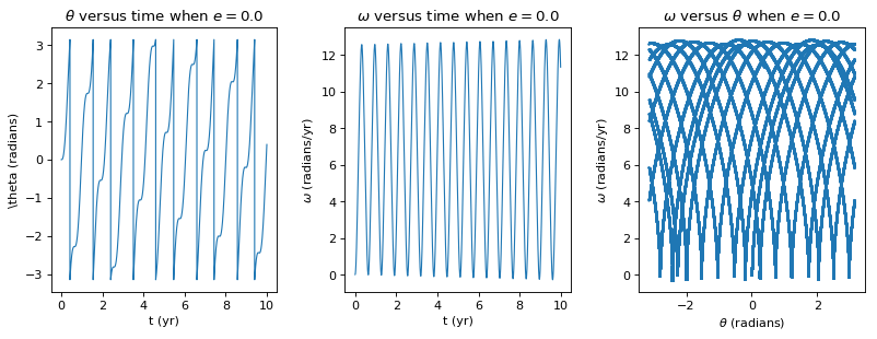
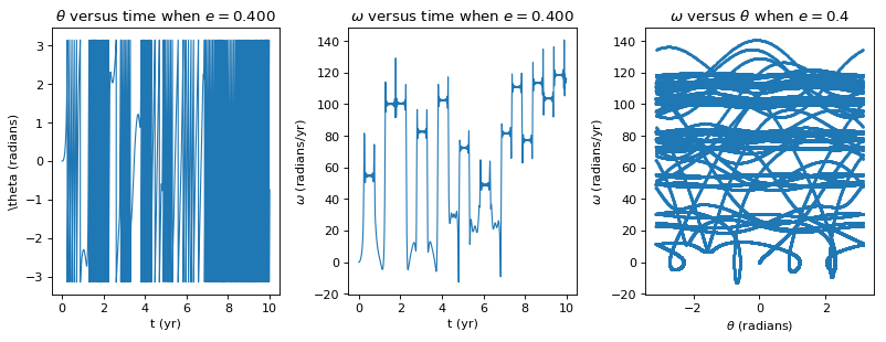
当离心率为 0 时,可以看到这是一个非混沌的系统,从角速度图像和相空间图可以很清楚的看出这一点。下面研究一下不同离心率情况下运动情况。
for e in (0.1, 0.2, 0.3, 0.4):
    a = hyperion(eccentricity = e)
    a.run()
    a.show()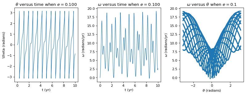
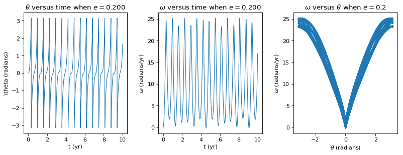
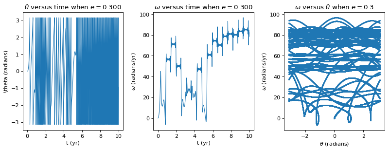
直观上很容易发现随着离心率的增大系统的混沌程度迅速增加,下面我们计算一下衡量混沌程度的 Lyapunov 指数来验证一下。
k = 221
pl.figure(figsize = (16,16), dpi=80)
for e in [0, 0.2, 0.4, 0.6]:
    a = hyperion(eccentricity = e, total_time=2)
    a.run()
    b = hyperion(eccentricity = e, initial_theta=0.001, total_time=2)
    b.run()
    delta_theta = b.theta_raw - a.theta_raw

    y = np.log(np.abs(delta_theta)) # 取对数后使用最小二乘法进行线性拟合
    func = np.polyfit(a.t, y, 1)
    y_fit = np.exp(func[0] * a.t + func[1])

    pl.subplot(k)
    pl.yscale('log')
    pl.plot(a.t, delta_theta, 'o', markersize = 1)
    pl.plot(a.t, y_fit, linewidth = 1.5)
    pl.xlabel('time(yr)')
    pl.ylabel(r'$\Delta \theta (radians)$')
    pl.title(r'$\Delta \theta$ verus time when when $e = %.1f$'% (a.e),)
    pl.text(1.5, 1e-6, '$\lambda=%.4f$'% func[0], size = 15)
    k += 1
pl.show()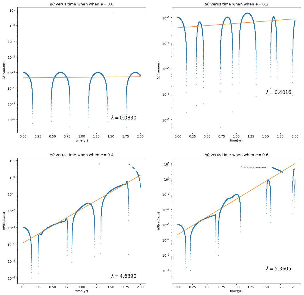
可以发现即使对于圆轨道,其 Lyapunov 指数仍然为正的,表明这个系统即使在圆轨道情况下也是略微混沌的。随着离心率的增加,Lyapunov 指数很明显是迅速增大的,这和我们之前的感觉是一致的。
5.7
Write two programs to solve the capacitor problem of Figure 5.6 and 5.7, one using the Jacobi method and one using the SOR algorithm. For a fixed accuracy (as set by the convergence test) compare the number of iterations,
, that each algorithm requires as a function of the number of grid elements, . Show that for the Jacobi method , while SOR . (非常正经的计算机算法研究方式^_^)
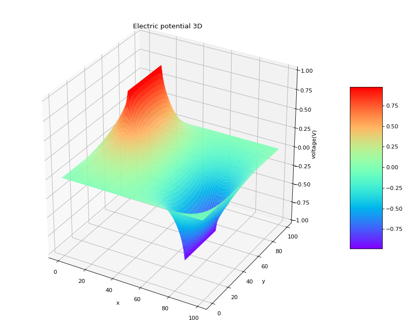
为了节约时间(生命),下面的代码已经包含了 SOR 方法和 Jacobi 方法,并直接使用 SOR 方法生成电场的图像。这里 SOR 方法的加速参数
import numpy as np
from matplotlib import pyplot as pl
from mpl_toolkits.mplot3d import Axes3D

class PDE(object):
    def __init__(self, length = 100):
        # 初始化边界条件
        self.v = np.zeros((length, length))
        self.l = length
        self.max = int(self.l * 0.7)
        self.min = int(self.l * 0.3)
        for i in range(self.l):
            for j in range(self.l):
                if self.min <= i <= self.max and j == self.min:
                    self.v[i, j] = 1
                elif self.min <= i <= self.max and j == self.max:
                    self.v[i, j] = -1

    def run(self, method = 'jacobi'):
        self.method = method
        self.delta_v = 1
        n_iter = 0
        while abs(self.delta_v) > self.l ** 2 * 1e-5:   # 判断是否已经收敛
            self.delta_v = 0
            n_iter += 1
            for i in range(self.l):
                for j in range(self.l):
                    if j == self.min and self.min <= i <= self.max:
                        pass
                    elif j == self.max and self.min <= i <= self.max:
                        pass
                    elif i == 0 or j == 0 or i == self.l-1 or j == self.l-1:
                        pass
                    else:
                        v_new = (self.v[i+1, j] + self.v[i-1, j] + self.v[i, j+1] + self.v[i, j-1]) / 4
                        if self.method == 'sor':
                            alpha = 2 / (1 + np.pi / self.l)
                            v_new = alpha * (v_new - self.v[i, j]) + self.v[i, j]
                        self.delta_v += abs(v_new - self.v[i, j])
                        self.v[i, j] = v_new
        return(n_iter)

    def show(self):
        X = np.arange(0, self.l)
        Y = np.arange(0, self.l)
        X, Y = np.meshgrid(X, Y)
        Z = self.v
        pl.figure(figsize = (10, 10), dpi = 80)
        CS = pl.contour(X, Y, Z, 30, alpha=1)
        pl.clabel(CS, inline=1, fontsize=10)
        pl.title('Electric potential 2D')
        pl.xlabel('x')
        pl.ylabel('y')

        figure = pl.figure(figsize = (10, 8), dpi = 80)
        ax = Axes3D(figure)
        surf = ax.plot_surface(X, Y, Z, rstride = 1, cstride = 1, cmap='rainbow')
        ax.set_xlabel('x')
        ax.set_ylabel('y')
        ax.set_zlabel('voltage(V)')
        ax.set_title('Electric potential 3D')
        figure.colorbar(surf, shrink=0.5, aspect=5)
        pl.show()

if __name__ == '__main__':
    a = PDE()
    a.run(method = 'sor')  # 这里直接使用 SOR 方法
    a.show()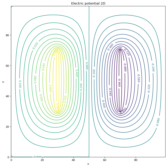
下面我们计算不同
n_sor = np.array([])
n_jacobi = np.array([])
leng = np.arange(10, 100, 5)
for l in leng:
    a = PDE(length = l)
    n_jacobi = np.append(n_jacobi, a.run())
    n_sor = np.append(n_sor, a.run(method = 'sor'))

func_jacobi = np.polyfit(leng, n_jacobi, 2)
n_fit_jacobi = func_jacobi[0] * leng ** 2 + func_jacobi[1] * leng + func_jacobi[2]
func_sor = np.polyfit(leng, n_sor, 1)
n_fit_sor = func_sor[0] * leng + func_sor[1]

pl.figure(figsize = (10, 10), dpi = 80)
pl.plot(leng, n_jacobi, 'ob')
pl.plot(leng, n_fit_jacobi, 'b', label = 'Jacobi method')
pl.plot(leng, n_sor, 'or')
pl.plot(leng, n_fit_sor, 'r', label = 'SOR method')
pl.xlabel('L')
pl.ylabel(r'$N_{iter}$')
pl.legend(loc = 'center right')
pl.text(10, 300, '$N_{Jacobi}\\approx%.2fL^2 + %.2fL %.2f$\n$N_{SOR}\\approx%.2fL %.2f$'% (func_jacobi[0], func_jacobi[1], func_jacobi[2], func_sor[0], func_sor[1]), size = 15)
pl.show()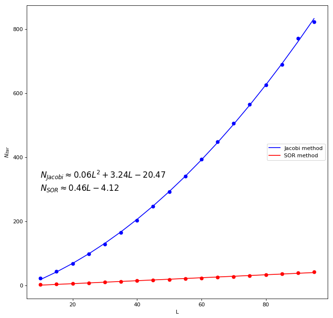
可以发现 SOR 方法的迭代次数是显著小于 Jacobi 方法的,根据曲线和拟合得到的参数可以看出 Jacobi 方法的迭代次数有