计算物理第十次作业
7.6
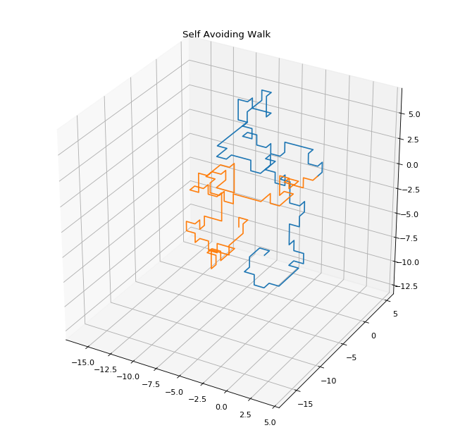
Simulate SAWs in three dimensions. Determine the vairation of
with step number and find the value of , where this parameter is defined through the relation (7.9). Compare your results with those in Figure 7.6. You should find that decreases for successively higher dimensions. (It is 1 in one dimension and 3/4 in two dimensions.) Can you explain this trend qualitatively?
为了保证随机行走每步的等可能性,这里采用的方法是检查生成的每一个新位置是否与已有位置重复,若重复,则重新生成,直到不重复。为了提高计算精度,模拟1000次后取平均值进行分析。
import time
import copy
import multiprocessing as mp
import numpy as np
import matplotlib.pyplot as pl
import mpl_toolkits.mplot3d.axes3d as ax3d
from scipy.optimize import curve_fit

def walk(last):
    # 随机挑选三维空间中的一个方向行走
    np.random.seed()
    while True:
        d = np.zeros(3)
        d[np.random.choice([0, 1, 2])] = np.random.choice([-1, 1])
        if (d != last).any():
            return d

def saw(steps = 500):
    while True:
        points = np.zeros((steps + 1, 3))
        points[1] = walk([0,0,0])
        i = 2
        while i <= steps:
            points[i] = points[i - 1] + walk(points[i - 2] - points[i - 1])
            if any(np.equal(points[:i-1], points[i]).all(1)):
                break
            i += 1
        if i == steps + 1:
            r2 = np.power(np.linalg.norm(points, axis=1),2)
            return points, r2
import time
import copy
import multiprocessing as mp
import numpy as np
import matplotlib.pyplot as pl
import mpl_toolkits.mplot3d.axes3d as ax3d
from scipy.optimize import curve_fit

def walk(last):
    # 随机挑选三维空间中的一个方向行走
    np.random.seed()
    while True:
        d = np.zeros(3)
        d[np.random.choice([0, 1, 2])] = np.random.choice([-1, 1])
        if (d != last).any():
            return d

def saw(steps = 50):
    while True:
        points = np.zeros((steps + 1, 3))
        points[1] = walk([0,0,0])
        i = 2
        while i <= steps:
            points[i] = points[i - 1] + walk(points[i - 2] - points[i - 1])
            if any(np.equal(points[:i-1], points[i]).all(1)):
                break
            i += 1
        if i == steps + 1:
            r2 = np.power(np.linalg.norm(points, axis=1),2)
            return points, r2

if __name__ == '__main__':
    t1 = time.time()
    args = [60] * 1000
    pool = mp.Pool()
    results = pool.map(saw, args)
    pool.close()
    pool.join()
    t2 = time.time()
    print('calucte time %.2f s'% (t2-t1))

    r2 = np.array([x[1] for x in results])
    results = np.array([x[0] for x in results])
    r2_mean = np.mean(r2, axis = 0)
    steps = np.arange(len(r2_mean))

    # 对结果进行拟合
    def func(x, a, b):
        return a * np.power(x, b)
    popt, pcov = curve_fit(func, steps, r2_mean)
    fit = func(steps, popt[0], popt[1])

    pl.figure(figsize = (10, 10), dpi = 80)
    pl.plot(steps, r2_mean, 'o', markersize = 1.5, label = '$<r^2>$')
    pl.plot(steps, fit, 'r', label = 'fit')
    pl.text(10, 1, r'$<r^2> \approx %.2f t^{%.3f}$'% (popt[0], popt[1]), size = 20)
    pl.title('Self Avoiding Walk')
    pl.xlabel('Number of Steps')
    pl.ylabel(r'$<r^2>$')
    pl.legend(loc = 'center right')
    pl.show()

    fig = pl.figure(figsize = (10, 10), dpi = 80)
    ax = fig.gca(projection='3d')
    ax.plot(results[0][:,0],results[0][:,1],results[0][:,2])
    ax.plot(results[1][:,0],results[1][:,1],results[1][:,2])
    pl.title('Self Avoiding Walk')
    pl.show()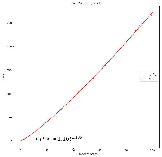
可以发现拟合的结果是
查找资料可知三维情况下理论值
另外在程序中进行了多进程的尝试,确实可以明显减少计算时间,但要注意应在随机开始时重新生成随机种子,否则会因为进程的复制而使得随机种子相同,造成失去随机的效果。
7.12
Calculate the entropy for the cream-in-your-coffee problem, and reproduce the results in Figure 7.16.
下面采用二维随机行走的方法模拟奶油的扩散,忽略掉粒子的相互作用,并且同一位置可以同时存在多个粒子。对于熵的计算采用单位长度的方格进行统计,即直接统计模拟粒子的坐标分布。
import copy
import numpy as np
import matplotlib.pyplot as pl

class cream(object):
    def __init__(self, total_time = 200, lenth = 200, particals = 1200):
        self.t = total_time
        self.n = particals
        self.l = lenth
        self.e = []
        self.d = int(self.n / 400)
        max_l = int(self.l / 2 + 10)
        min_l = int(self.l / 2 - 10)
        grid = np.mgrid[min_l:max_l, min_l:max_l]
        points = np.vstack(map(np.ravel, grid)).T
        self.points = np.tile(points, (self.d, 1))

    def run(self):
        t = 0
        diff, counts = np.unique(self.points, axis = 0, return_counts=True)
        self.diff = [copy.deepcopy(diff)]
        self.counts = [copy.deepcopy(counts)]
        while t < self.t:
            old = copy.deepcopy(self.points)
            for i in range(self.n):
                d = np.zeros(2)
                d[np.random.choice((0, 1))] = np.random.choice((-1, 1))
                self.points[i] = old[i] + d
            t += 1
            diff, counts = np.unique(self.points, axis = 0, return_counts=True)
            self.e.append(np.sum(- counts / self.n * np.log(counts / self.n)))
            if t in [100, 500, 1000]:
                self.diff.append(copy.deepcopy(diff))
                self.counts.append(copy.deepcopy(counts))

    def show(self):
        pl.figure(figsize = (10, 10), dpi = 80)
        k = 221
        i = 0
        for t in [0, 100, 500, 1000]:
            pl.subplot(k)
            pl.scatter(self.diff[i][:,0], self.diff[i][:,1], c = self.counts[i], cmap='rainbow', s = 2)
            pl.xlim(0, 200)
            pl.ylim(0, 200)
            pl.title('Cream in coffee t = %d'% t)
            pl.xlabel('x')
            pl.ylabel('y')
            k += 1
            i += 1
        pl.colorbar(orientation='horizontal')
        pl.show()

        pl.figure(figsize = (10, 10), dpi = 80)
        pl.plot(range(self.t), self.e)
        pl.xlabel('time(steps)')
        pl.ylabel('Entropy')
        pl.title('Entropy versus time')
        pl.show()

if __name__ == '__main__':
    a = cream(total_time = 2000, particals=800)
    a.run()
    a.show()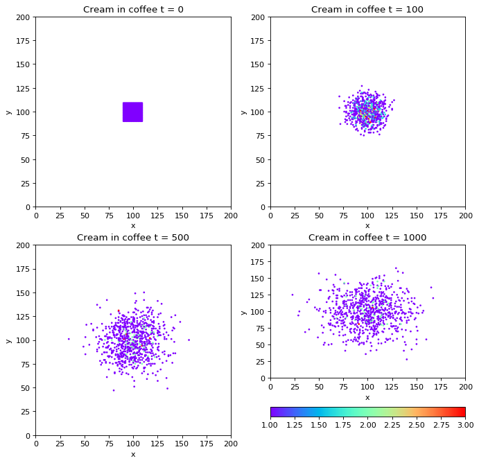
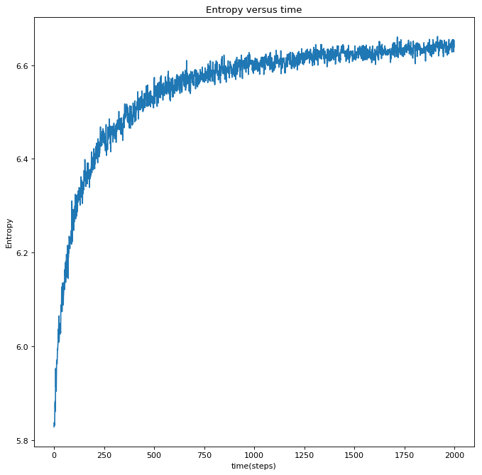
可以看到模拟计算得到的熵值是逐渐增大,并且增长趋势是减缓的,这和课本以及热统的知识相符,即系统会达到熵最大的平衡状态。由于划分的网格比较细,因此可以发现熵的波动幅度大于课本上的图7.16(使用的是8×8方格)。